
Short Answer
Pivot tables are powerful tools for data analysis, delivering quick insights with minimal effort. However, when dealing with large datasets, identifying the top 10 results can often be a tedious task. This guide offers a fresh perspective on how to effortlessly extract and display the top 10 entries in pivot tables, transforming your data analysis experience and saving you valuable time. Get ready to elevate your Excel skills and make your data work smarter.
1. Utilize the Value Filters Feature
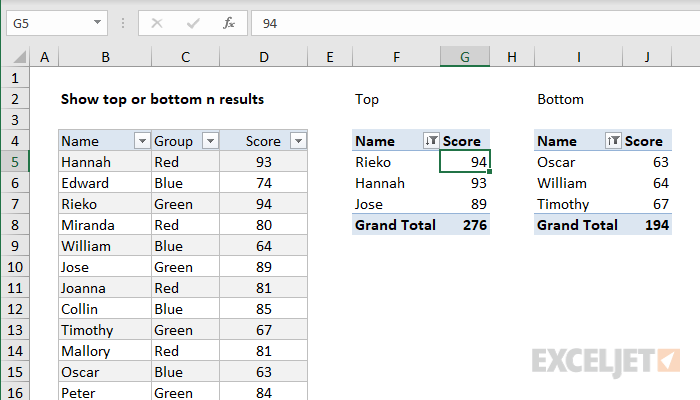
The simplest way to show the top 10 results is by applying a Value Filter. Right-click on the field in the pivot table row or column labels, select “Value Filters,” then choose “Top 10.” This method instantly narrows down your data to the highest values, whether it’s top 10 items, customers, or periods.
2. Customize the Number of Items in Value Filters
While the default is set to 10, Excel allows you to adjust this number. In the Value Filter dialog box, change the number to any quantity you’d prefer, such as top 5 or top 20, giving you flexibility based on your analytical needs.
3. Filter by Top or Bottom Items
Value Filters not only show top values but also bottom results. You can switch between “Top” and “Bottom” in the filter options, broadening your ability to detect underperforming elements or lower-ranking entries.
4. Add a Rank Column Using Calculated Fields
For more complex scenarios, create a calculated field that ranks items based on the values. This approach lets you display ranks directly in your pivot table, making it easy to visually identify top performers without manual filtering.
5. Use the Filter Pane in Newer Excel Versions
The Filter Pane offers an intuitive way to filter fields. You can apply number filters within it to quickly select the top 10 items, streamlining the process and providing a more modern interface than traditional filter menus.
6. Implement Slicers to Control Filtering
Slicers provide interactive filters with clickable buttons. Setting them to filter top 10 items allows dynamic adjustment and offers an engaging way to explore high-ranking data points alongside your pivot table.
7. Combine Top 10 Filters with Date Grouping
Grouping dates (months, quarters, years) in your pivot table and then applying top 10 value filters can reveal trends over time, highlighting the best performers within specific periods for deeper insights.
8. Sort Pivot Table for Visual Clarity
Sorting data in descending order before applying the top 10 filter improves readability. It ensures that the pivot table lists the highest values at the top, reinforcing the focus on key performers in your dataset.
9. Use Advanced Filter Options for Multiple Conditions
Excel supports complex filtering criteria. You can combine top 10 filters with other conditions (e.g., product category or region) to pinpoint top performers within subsets of your data, resulting in targeted analysis.
10. Export Filtered Data for Reporting
After isolating the top 10 items, consider copying the filtered pivot table to a new sheet or workbook. This preserves your results for reporting or presentation purposes without risking accidental changes to the original data.
11. Leverage Power Pivot for Large Datasets
If you’re handling massive data, Power Pivot offers more advanced filtering options and better performance. You can create measures and calculated columns to dynamically show the top 10 results with greater flexibility.
12. Refresh and Update Filters Regularly
Pivot tables don’t automatically update filters when your source data changes. Always refresh your pivot table and confirm your top 10 filter remains intact to maintain accurate and current results.
13. Use Conditional Formatting to Highlight Top 10
Instead of filtering, apply conditional formatting rules to highlight the top 10 values in your pivot table. This method leaves the full dataset visible while visually emphasizing the highest values for quick reference.
14. Utilize the GETPIVOTDATA Function for Custom Reports
Combine pivot tables with the GETPIVOTDATA function in Excel to extract and display top 10 results dynamically in summary reports, enhancing your ability to present filtered data outside the pivot table environment.
15. Avoid Common Pitfalls with Cached Data
Remember that pivot tables cache data, which can affect filtering accuracy. Clear cache or recreate pivot tables if filtering behaves unexpectedly after data updates to ensure reliable top 10 displays.
FAQ
How do I show the top 10 results in a pivot table?
Use the Value Filters feature by right-clicking the pivot table field, selecting ‘Value Filters,’ then choosing ‘Top 10’ to display the highest values.
Can I customize the number of top items displayed in a pivot table?
Yes, in the Value Filter dialog box, you can change the default number from 10 to any number you prefer, such as top 5 or top 20.
What is the benefit of using slicers with top 10 filters?
Slicers provide an interactive and user-friendly way to filter pivot table data dynamically, allowing easy adjustment of top 10 items displayed.
How do I ensure my top 10 filters remain accurate when data changes?
Always refresh your pivot table after updating source data to maintain filter accuracy and ensure the top 10 results are current.
Can I highlight top 10 values without filtering pivot tables?
Yes, applying conditional formatting to highlight top 10 values visually emphasizes key data points without hiding other data.
FAQ
How do I show the top 10 results in a pivot table?
You can apply a Value Filter in your pivot table by right-clicking the field in row or column labels, selecting ‘Value Filters,’ and choosing ‘Top 10’ to display the highest values.
Can I customize the number of top items displayed in a pivot table?
Yes, in the Value Filter dialog box, you can change the default number 10 to any number like 5 or 20 to suit your needs.
How do slicers help in showing top 10 results?
Slicers provide interactive buttons to filter pivot table data dynamically, allowing you to adjust and explore top-ranking items easily.
What should I do if pivot table filters don’t update with new data?
You should refresh your pivot table regularly to ensure filters remain accurate and data is current.
Can I highlight top 10 values without filtering them out?
Yes, using conditional formatting rules in Excel, you can visually emphasize the top 10 values while keeping all data visible.
FAQ
How do I show the top 10 results in an Excel pivot table?
You can use the Value Filters feature in the pivot table by right-clicking the field, selecting ‘Value Filters,’ and choosing ‘Top 10’ to display the highest values.
Can I customize the number of top items shown in a pivot table?
Yes, Excel allows you to change the default top 10 number to any value you prefer within the Value Filter dialog box.
How can I highlight top 10 values without filtering out other data?
You can apply conditional formatting rules to visually highlight the top 10 values while keeping the full dataset visible.
What should I do if my pivot table filters do not update after data changes?
Always refresh your pivot table after updating the source data to ensure filters and top 10 results are current.





Leave a Reply